# visualizeR  > What a color! What a viz!
`visualizeR` proposes some utils to get REACH and AGORA colors,
ready-to-go color palettes, and a few visualization functions
(horizontal hist graph for instance).
## Installation
You can install the last version of visualizeR from
[GitHub](https://github.com/) with:
``` r
# install.packages("devtools")
devtools::install_github("gnoblet/visualizeR", build_vignettes = TRUE)
```
## Roadmap
Roadmap is as follows:
- [x] Add IMPACT’s colors
- [x] Add all color palettes from the internal documentation
- [ ] There remains to be added more-than-7-color palettes and black
color palettes
- [ ] Add new types of visualization (e.g. dumbbell plot)
- [ ] Use examples
- [ ] Add some ease-map functions
- [ ] Add some interactive functions (maps and graphs)
## Request
Please, do not hesitate to pull request any new viz or colors or color
palettes, or to email request any change
( or ).
## Example 1: extracting colors
Color palettes for REACH, AGORA and IMPACT are available. Functions to
access colors and palettes are `cols_initiative()` or
`pal_initiative()`. For now, the initiative with the most colors and
color palettes is REACH. Feel free to pull requests new AGORA and IMPACT
colors.
``` r
library(visualizeR)
# Get all saved REACH colors, named
cols_reach(unnamed = F)[1:10]
#> white black main_grey main_red main_lt_grey main_beige
#> "#FFFFFF" "#000000" "#58585A" "#EE5859" "#C7C8CA" "#D2CBB8"
#> iroise_1 iroise_2 iroise_3 iroise_4
#> "#DFECEF" "#B1D7E0" "#699DA3" "#236A7A"
# Extract a color palette as hexadecimal codes and reversed
pal_reach(palette = "main", reversed = TRUE, color_ramp_palette = FALSE)
#> [1] "#58585A" "#EE5859" "#C7C8CA" "#D2CBB8"
# Get all color palettes names
pal_reach(show_palettes = T)
#> [1] "main" "primary" "secondary" "two_dots"
#> [5] "two_dots_flashy" "red_main" "red_main_5" "red_alt"
#> [9] "red_alt_5" "iroise" "iroise_5" "discrete_6"
#> [13] "red_2" "red_3" "red_4" "red_5"
#> [17] "red_6" "red_7" "green_2" "green_3"
#> [21] "green_4" "green_5" "green_6" "green_7"
#> [25] "artichoke_2" "artichoke_3" "artichoke_4" "artichoke_5"
#> [29] "artichoke_6" "artichoke_7" "blue_2" "blue_3"
#> [33] "blue_4" "blue_5" "blue_6" "blue_7"
```
## Example 2: Bar chart, already REACH themed
``` r
library(visualizeR)
library(palmerpenguins)
library(dplyr)
df <- penguins |>
group_by(island, species) |>
summarize(
mean_bl = mean(bill_length_mm, na.rm = T),
mean_fl = mean(flipper_length_mm, na.rm = T)) |>
ungroup()
# Simple bar chart by group
bar_reach(df, mean_bl, island, species, percent = FALSE, x_title = "Mean of bill length")
```
> What a color! What a viz!
`visualizeR` proposes some utils to get REACH and AGORA colors,
ready-to-go color palettes, and a few visualization functions
(horizontal hist graph for instance).
## Installation
You can install the last version of visualizeR from
[GitHub](https://github.com/) with:
``` r
# install.packages("devtools")
devtools::install_github("gnoblet/visualizeR", build_vignettes = TRUE)
```
## Roadmap
Roadmap is as follows:
- [x] Add IMPACT’s colors
- [x] Add all color palettes from the internal documentation
- [ ] There remains to be added more-than-7-color palettes and black
color palettes
- [ ] Add new types of visualization (e.g. dumbbell plot)
- [ ] Use examples
- [ ] Add some ease-map functions
- [ ] Add some interactive functions (maps and graphs)
## Request
Please, do not hesitate to pull request any new viz or colors or color
palettes, or to email request any change
( or ).
## Example 1: extracting colors
Color palettes for REACH, AGORA and IMPACT are available. Functions to
access colors and palettes are `cols_initiative()` or
`pal_initiative()`. For now, the initiative with the most colors and
color palettes is REACH. Feel free to pull requests new AGORA and IMPACT
colors.
``` r
library(visualizeR)
# Get all saved REACH colors, named
cols_reach(unnamed = F)[1:10]
#> white black main_grey main_red main_lt_grey main_beige
#> "#FFFFFF" "#000000" "#58585A" "#EE5859" "#C7C8CA" "#D2CBB8"
#> iroise_1 iroise_2 iroise_3 iroise_4
#> "#DFECEF" "#B1D7E0" "#699DA3" "#236A7A"
# Extract a color palette as hexadecimal codes and reversed
pal_reach(palette = "main", reversed = TRUE, color_ramp_palette = FALSE)
#> [1] "#58585A" "#EE5859" "#C7C8CA" "#D2CBB8"
# Get all color palettes names
pal_reach(show_palettes = T)
#> [1] "main" "primary" "secondary" "two_dots"
#> [5] "two_dots_flashy" "red_main" "red_main_5" "red_alt"
#> [9] "red_alt_5" "iroise" "iroise_5" "discrete_6"
#> [13] "red_2" "red_3" "red_4" "red_5"
#> [17] "red_6" "red_7" "green_2" "green_3"
#> [21] "green_4" "green_5" "green_6" "green_7"
#> [25] "artichoke_2" "artichoke_3" "artichoke_4" "artichoke_5"
#> [29] "artichoke_6" "artichoke_7" "blue_2" "blue_3"
#> [33] "blue_4" "blue_5" "blue_6" "blue_7"
```
## Example 2: Bar chart, already REACH themed
``` r
library(visualizeR)
library(palmerpenguins)
library(dplyr)
df <- penguins |>
group_by(island, species) |>
summarize(
mean_bl = mean(bill_length_mm, na.rm = T),
mean_fl = mean(flipper_length_mm, na.rm = T)) |>
ungroup()
# Simple bar chart by group
bar_reach(df, mean_bl, island, species, percent = FALSE, x_title = "Mean of bill length")
```
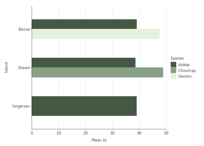
 ``` r
# Using another color palette
bar_reach(df, mean_bl, island, species, percent = FALSE, palette = "artichoke_3", legend_rev = TRUE)
```
``` r
# Using another color palette
bar_reach(df, mean_bl, island, species, percent = FALSE, palette = "artichoke_3", legend_rev = TRUE)
```
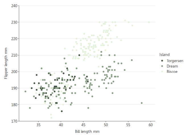
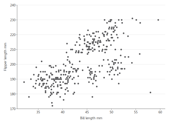
 ## Example 3: Point chart, already REACH themed
At this stage, `point_reach()` only supports categorical grouping colors
with the `group` arg.
``` r
# Simple point chart
point_reach(penguins, bill_length_mm, flipper_length_mm)
```
## Example 3: Point chart, already REACH themed
At this stage, `point_reach()` only supports categorical grouping colors
with the `group` arg.
``` r
# Simple point chart
point_reach(penguins, bill_length_mm, flipper_length_mm)
```
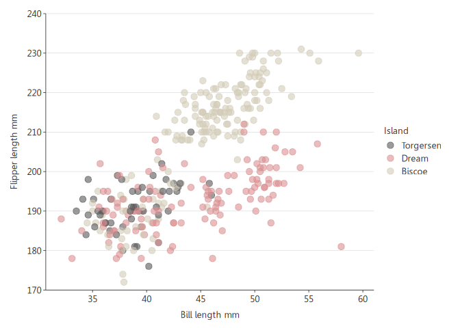
 ``` r
# Point chart with grouping colors, greater dot size, some transparency, reversed color palette
point_reach(penguins, bill_length_mm, flipper_length_mm, island, alpha = 0.6, size = 3, reverse = TRUE)
```
``` r
# Point chart with grouping colors, greater dot size, some transparency, reversed color palette
point_reach(penguins, bill_length_mm, flipper_length_mm, island, alpha = 0.6, size = 3, reverse = TRUE)
```
 ``` r
# Using another color palettes
point_reach(penguins, bill_length_mm, flipper_length_mm, island, palette = "artichoke_3")
```
``` r
# Using another color palettes
point_reach(penguins, bill_length_mm, flipper_length_mm, island, palette = "artichoke_3")
```